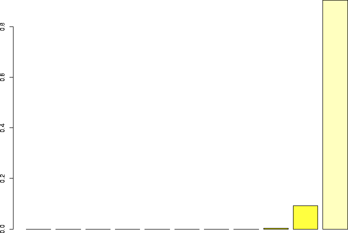
N=10, p=0.99
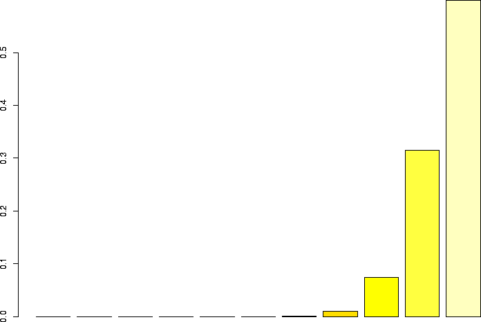
N=10, p=0.95
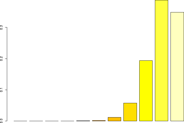
N=10, p=0.9
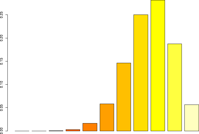
N=10, p=0.75
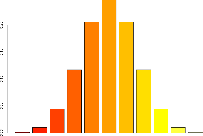
N=10, p=0.5
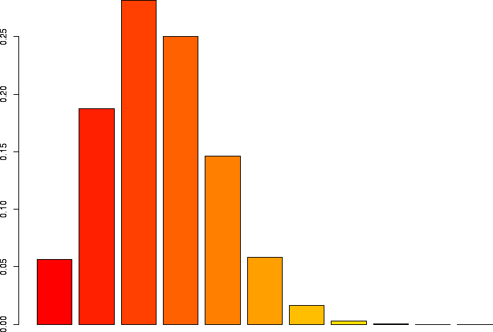
N=10, p=0.25

N=10, p=0.1
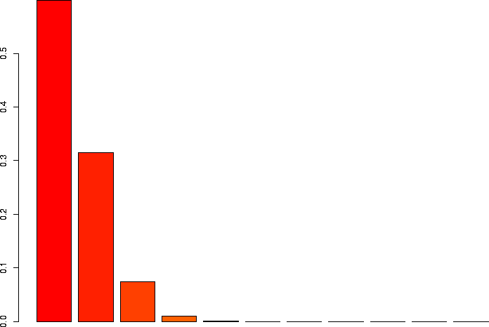
N=10, p=0.05
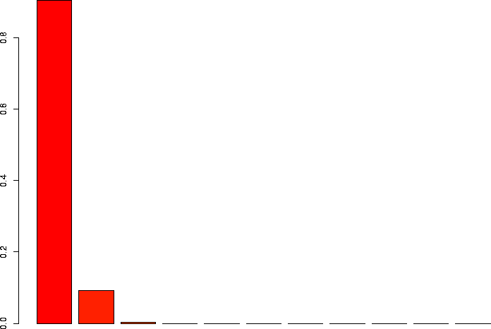
N=10, p=0.01

| Home About us Mathematical Epidemiology Rweb EPITools Statistics Notes Web Design Search Contact us |
Let's switch gears a little and do an example. You've probably seen how to do confidence intervals for proportions using the normal approximation to the binomial. But sometimes this leads to problems, especially when the numbers aren't large (so the approximation does not work so well).
Before we show how to compute confidence intervals, however, let's review the binomial distribution itself, and in the process, learn more about the random number functions provided by R.
A Bernoulli trial is a random variable with two outcomes, conventionally
called success (1) and failure (0). If you perform N
Bernoulli trials, each with success probability p, the number X
of successes is a binomial random variable. The expected number of
successes is Np, the variance of X is Np(1-p), and the
probability that X equals x is given by
(N!/(x!(N-x)!))px(1-p)N-x.
This probability function can be computed in R using the function dbinom. How about tossing a single fair coin, one time? Here there is only one Bernoulli trial, so we have a binomial with N equal to one. Since the coin is fair, the probability of a head is 0.5, so if we think of heads as a success, the success probability p is 0.5. And of course the success probability is 0.5 if we call tails a success also. The number of heads is X, and we want to know the probability that X is 0. So using dbinom:
> dbinom(0,size=1,prob=0.5) [1] 0.5 |
> dbinom(0,1,0.5) [1] 0.5 |
> dbinom(0,size=2,prob=0.5) [1] 0.25 |
> dbinom(1,size=2,prob=0.5) [1] 0.5 |
Let's toss the two independent fair coins again and ask what the chance of getting two heads is. You know it; it's 0.25:
> dbinom(2,size=2,prob=0.5) [1] 0.25 |
> dbinom(3,size=2,prob=0.5) [1] 0 |
Another example: suppose that 51 individuals receive a needlestick injury with hepatitis-C positive blood, and that the probability of infection from such an injury is 0.03. What is the probability that no individuals are infected? Here, let X be the number of individuals infected. There are 51 trials (N=51), and we will suppose these are independent trials. (Can this be taken for granted?) Let's call infection the "success" and non-infection the "failure", so that the success probability p=0.03. So now the number of infected individuals is a binomial random variable with parameters N and p. We want to know the probability that X equals zero. We could use the formula in the above paragraph explicitly, but this formula is available through dbinom:
> dbinom(0,size=51,prob=0.03) [1] 0.2115234 |
Suppose that a person has ten sex partners chosen "independently and at random" from a population with a prevalence of HIV of 0.4 (40%). Now suppose that the probability of becoming infected during a partnership with an infected partner (assuming that unprotected sex happens) is 0.1. What is the chance of becoming infected? Here, we use a Bernoulli risk model (Grant et al 1987); each partnership is assumed to be an independent trial. The chance of becoming infected (assuming that partner HIV status and infectivity are independent; is this reasonable?) would be 0.4 × 0.1 = 0.04. Let's call the number of times a person would get infected X, and call "getting infected" the "success"; then we have 10 independent Bernoulli trials each with success probability 0.04. If X is 1, 2, 3, 4, 5, 6, 7, 8, 9, or 10, then the person gets infected; if X is 0, the person does not. It is simpler to determine the chance of not getting zero (one minus the chance of getting zero) than it is to compute the chance of getting a number between 1 and 10 (inclusive):
> 1 - dbinom(0,size=10,prob=0.04) [1] 0.3351674 |
The function dbinom is vectorized, so we can compute a lot of these probabilities at once. Let's compute the chance of getting zero, one or two heads in two tosses of fair coins independently:
> dbinom(0:2,size=2,prob=0.5) [1] 0.25 0.50 0.25 |
Let's look at all the possibilities for the hepatitis example. Here, the size was 51, the success probability was 0.03; the possible outcomes range from 0 to 51:
> barplot(dbinom(0:51,size=51,prob=0.03)) |
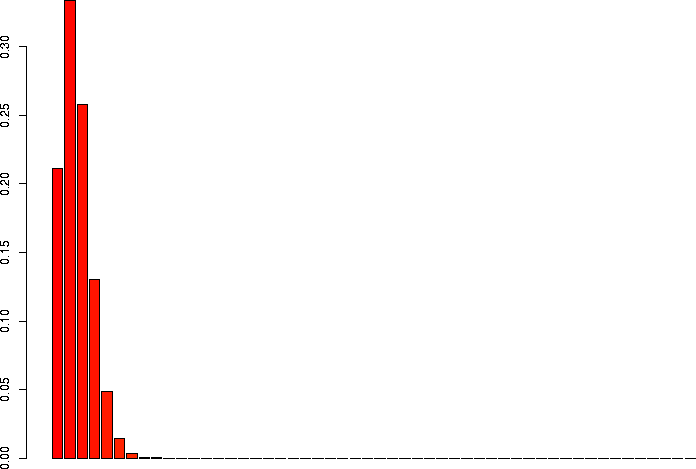
> sum(dbinom(9:51,size=51,prob=0.03)) [1] 1.910332e-05 > 1-sum(dbinom(0:8,size=51,prob=0.03)) [1] 1.910332e-05 > dbinom(51,size=51,prob=0.03) [1] 2.153694e-78 |
Let's linger a little more and look at some more binomial distributions. Let's look at a binomial probability function with N=10, but different values of p:
 N=10, p=0.99 |
 N=10, p=0.95 |
 N=10, p=0.9 |
 N=10, p=0.75 |
 N=10, p=0.5 |
 N=10, p=0.25 |
 N=10, p=0.1 |
 N=10, p=0.05 |
 N=10, p=0.01 |
I'd also like to take a look at several of these keeping p the same, but varying N.
> barplot(dbinom(0:3,size=3,prob=0.1)) > barplot(dbinom(0:10,size=10,prob=0.1)) > barplot(dbinom(0:30,size=30,prob=0.1)) > barplot(dbinom(0:100,size=100,prob=0.1)) > barplot(dbinom(0:300,size=300,prob=0.1)) > barplot(dbinom(0:1000,size=1000,prob=0.1)) |
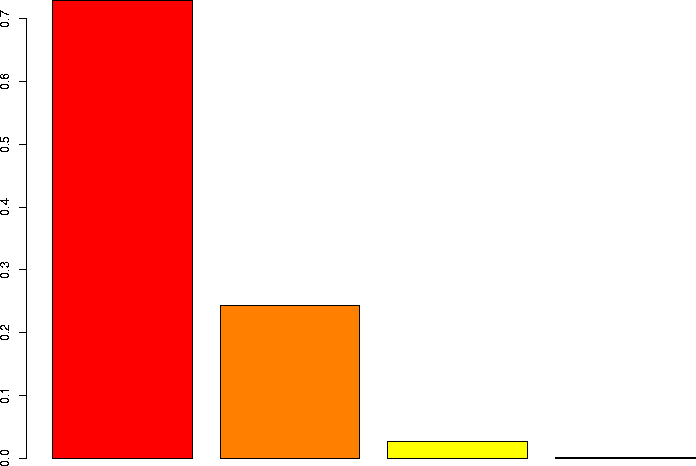 N=3, p=0.1 |
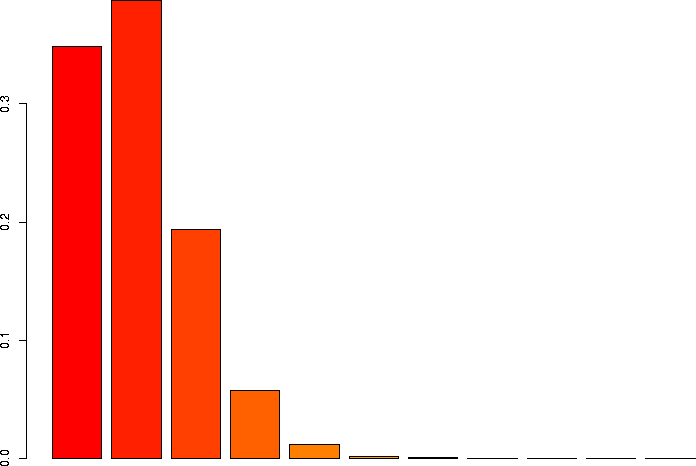 N=10, p=0.1 |
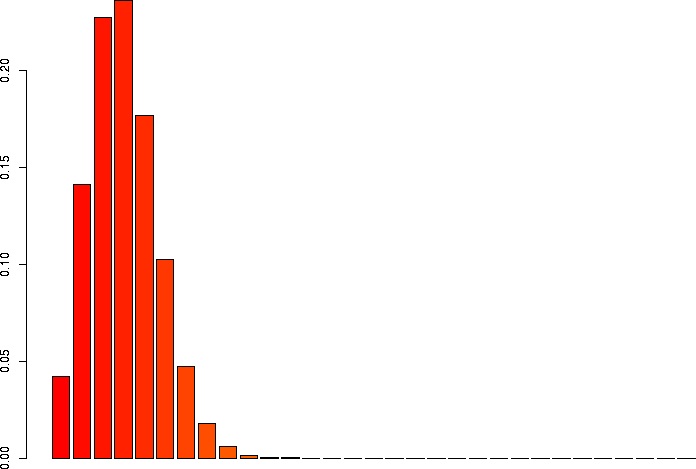 N=30, p=0.1 |
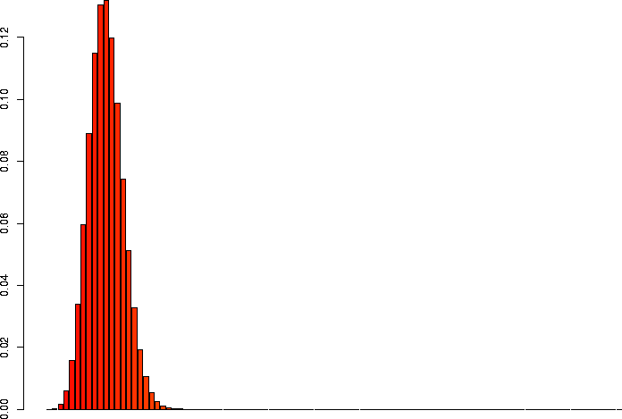 N=100, p=0.1 |
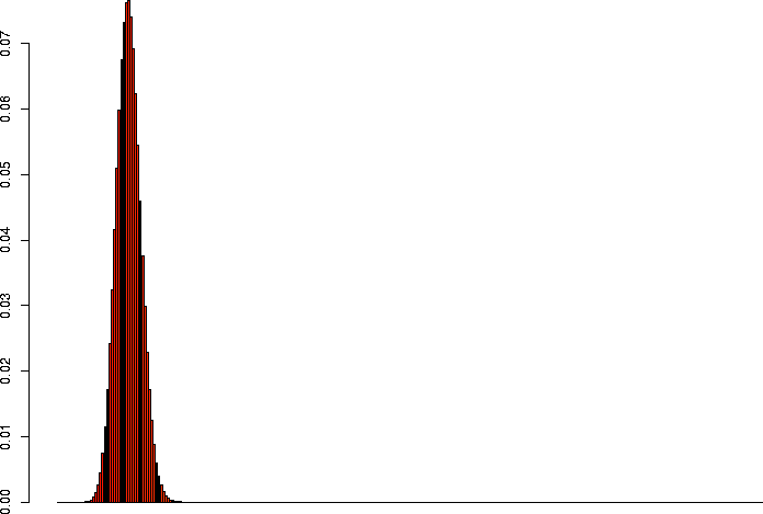 N=300, p=0.1 |
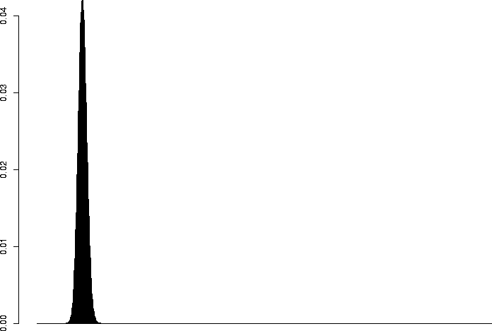 N=1000, p=0.1 |
Let's think about estimation a bit. If you don't know the success probability, but want to estimate it from data, we know our best estimate is the observed success fraction, X/N. This is traditionally denoted as a p with a circumflex on top of it. Unfortunately the most common HTML encoding doesn't include a p with this accent on it, although we can accent the vowels. So we'll break from tradition and just use a capital P to be X/N, the observed success fraction. We say that P estimates p, i.e. the observed success fraction estimates the unknown true success probability.
Now, what is the expected value of P? If we keep doing the binomial experiment over and over again, on average, what is P? Notice that N is constant each time; it is a fixed parameter. But X is random; each time we do the experiment, we get a different number of successes. We know E[P] = E[X/N] just by definition, and since N is constant, we can just move it out. So E[P]=E[X]/N (in general, if you (say) halve all the random values, you halve the average, and so forth). But the expected value of X is Np as we said. So E[P]=Np/N=p. The expected value of P is p; on average, you expect the estimator to equal the value it's estimating. This is a nice property the mathematicians call "unbiasedness". So the observed success fraction is an unbiased estimator of p.
The Weak Law of Large Numbers tells us something too. We know at least from simulation (that you just saw) that if N gets big, the success fraction is close to the probability. (In fact, this convergence is the basis of the very definition of probability as the frequentists see it.) What is the chance that there is a "meaningful" difference between P and p? If we pick some number like E, and ask what the chance that |P-p|>E, the Weak Law of Large Numbers tells us that we can make this chance as small as we like if we are willing to make N large enough. This fact makes P what the mathematicians call a consistent estimator of p.
I want to talk about an important property of P, the observed success fraction. Let's return for a moment to the experiment I discussed before, in which 3 infections were observed out of 51 needlestick injuries with Hepatitis C positive blood. In reality, we don't know the probability of infection from any first principles. And it would differ with such things as the size of the needle, depth of injury, and so forth. So this probability would probably differ in different populations. We believe that the observed success proportion 3/51=0.0588 is a good estimate of the unknown true probability.
Let's look at the probability of seeing 3 (exactly 3) infections out of 51 under different circumstances. Suppose the infection probability were really 0.01. Then
> dbinom(3,prob=0.01,size=51) [1] 0.01285507 |
> dbinom(3,prob=0.001,size=51) [1] 1.984853e-05 |
Now, let's plot the probability of seeing 3 infections out of 51, for various values of the infection probability p (the success probability in the binomial). We're picking one particular probability out of a distribution and plotting it as we change p, so of course this is not a probability distribution. It is the probability of the data (3) as a function of the unknown parameter p, and this is called the likelihood function:
> xs <- seq(0.001,0.999,by=0.001) > plot(xs,dbinom(3,prob=xs,size=51),type="l") |
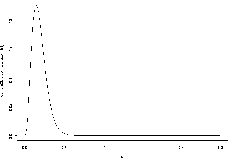
Let's see how we could find this maximum value in R. We have a one-dimensional function that we want to find the maximum value of. In other words, conceptually, we have a function that takes a value of p, and gives us the probability of the data for that value of p. The function we will use is called optimize, and it is good for one-dimensional optimization. For multidimensional optimization, we use optim. So let's see this work:
> 3/51 [1] 0.05882353 > fn <- function(pp) dbinom(3,prob=pp,size=51) > optimize(fn,interval=c(0.0001,0.9999),maximum=TRUE) $maximum [1] 0.05882187 $objective [1] 0.2309134 |
It turns out that P, the observed success fraction, is in fact the true maximum likelihood estimate of the unknown success probability. This can be shown by taking the logarithm (to make the math easier) of the probability function, and setting the first derivative to zero, etc. We're not going to show that in this class. Just note that the use of optimize gave us a reasonably close approximation.
Now, we've already seen that if p were 0.001, there would be an about 2 in 100000 chance of seeing the data we saw. Is it plausible that the true probability could be as small as 0.001? So let's think about what we might see if p were 0.001. What would it take to change our mind? If p were 0.001, then the probability of seeing 0 infections is 0.9503, seeing 1 infection is 0.04851, of seeing 2 infections is 0.0012, etc. The idea is that if the success probability were small, you expect to see a small number of successes. If the infection probability is small, you should see a small number of infections. If you see a large enough number of infections, maybe you should change your mind about the probability being small.
Formally, we could call p=0.001 the null hypothesis. The data we will have is the number of infections out of the study population. We can calculate the fraction of successes (infections), P=X/N using the notation from before; under the null hypothesis, X has a binomial distribution with parameters p=0.001 and N=51. We know that if p is small, we had better see a small P. So a big P will lead us to reject the null hypothesis, and in this case, what we'll reject is p=0.001.
So how big is big? Remember, any big value will lead us to reject the hypothesis. We're interested in things like P(X>=x for various values of x (and here the capital P just refers to probability). So in other words, if some x is so big we'd give up on p=0.001, then something even bigger is even worse as far as the credibility of p=0.001 is concerned.
R conveniently computes the cumulative distribution function, P(X<=x) using pbinom. This saves us the trouble of using sum on a range. And there is an analogous version for many continuous variables like the normal (e.g. pnorm).
> pbinom(0,prob=0.001,size=51) [1] 0.9502544 > pbinom(1,prob=0.001,size=51) [1] 0.998766 > pbinom(2,prob=0.001,size=51) [1] 0.99998 > pbinom(3,prob=0.001,size=51) [1] 0.9999998 > pbinom(3,prob=0.001,size=51)-sum(dbinom(0:3,prob=0.001,size=51)) [1] 0 |
Let's write a function to compute P(X>=x) for binomial random variables. To be x or bigger is to not be x-1 or smaller; the binomial has no values in between integers:
pr.ge.binom <- function(xx,prob,size) {
  1-pbinom(xx-1,prob=prob,size=size)
|
So how big would be too big? We could decide in advance that the smallest value of x so that P(X>=x) is less than or equal to 0.05 is going to be the cutoff. Let's take a look at some of this:
> pr.ge.binom <- function(xx,prob,size) {
+   1-pbinom(xx-1,prob=prob,size=size)
+ }
> for (xx in 0:10) {
+   cat("xx=")
+   cat(xx)
+   cat("; and P(X>=x)=")
+   cat(pr.ge.binom(xx,prob=0.001,size=51))
+   cat("\n")
+ }
xx=0; and P(X>=x)=1
xx=1; and P(X>=x)=0.04974558
xx=2; and P(X>=x)=0.001234090
xx=3; and P(X>=x)=2.008922e-05
xx=4; and P(X>=x)=2.406816e-07
xx=5; and P(X>=x)=2.260727e-09
xx=6; and P(X>=x)=1.732803e-11
xx=7; and P(X>=x)=1.113554e-13
xx=8; and P(X>=x)=6.661338e-16
xx=9; and P(X>=x)=0
xx=10; and P(X>=x)=0
|
> sum(dbinom(9:51,prob=0.001,size=51)) [1] 2.92943e-18 |
If we're doing a one-tailed test with significance probability 0.05, then we would reject the hypothesis p=0.001 even if we see one single infection out of 51. If the probability really were 0.001, and we did this experiment of looking at 51 random independent subjects over and over again, rejecting the hypothesis whenever we see 1 or more infections, then we'll be wrong, in the long run, 4.97% of the time. If we wanted a smaller Type I error rate, such as 1%, we would have to stop rejecting the hypothesis if we see one single infection. To have a type I error rate no bigger than 1%, we would have to reject only when we see 2 or more infections (and our type I error rate is then what?).
Question: what if we believe that the true infection probability is smaller than 0.001, and we have 51 subjects. Why can't we ever conclude based on this sample size that 0.001 is too big?
Let's go back to 3 infections out of 51 injuries. We agree that 3/51=0.058 is the best estimate. But how small could the probability be, and be consistent with our observation? How big could it be? Let's say that we will use a two-sided test with 2.5% of the probability (or as close as we can) on each side.
We know that if our hypothesis were p=0.001, we would reject the hypothesis if we saw anything bigger than 2 (with a 0.12% error rate). But what about a bigger p? Let's look at a few:
> sum(dbinom(3:51,size=51,prob=0.01)) [1] 0.01457345 > sum(dbinom(3:51,size=51,prob=0.005)) [1] 0.002175924 > sum(dbinom(3:51,size=51,prob=0.02)) [1] 0.08214377 > sum(dbinom(3:51,size=51,prob=0.015)) [1] 0.0412478 |
We can use the function uniroot to find numbers like this in one dimension:
> fn <- function(pp) {
+   sum(dbinom(3:51,size=51,prob=pp))-0.025
+ }
> uniroot(fn,interval=c(0.00001,0.99999))
$root
[1] 0.01230370

$f.root
[1] 2.407805e-05

$iter
[1] 7

$estim.prec
[1] 6.103516e-05

> 1-pbinom(2,size=51,prob=0.0123)
[1] 0.02500476
|
Here, we saw an example of root finding in action. Lots of things could go wrong with root finding: there might not be a root, or there might be more than one root in the interval, or the function might be irregular or strange. So you can never take this sort of thing for granted, even in one dimension (with one argument that can vary). The function uniroot is R's builtin function for helping you do one-dimensional root finding, for purposes like this one. When you use it, always plot your function and make sure you understand the behavior of the function whose root you want. Here is a plot of the function we just looked at:
> fn <- function(pp){1-pbinom(2,size=51,prob=pp)-0.025}
> xx <- seq(0.001,0.02,by=0.001)
> plot(xx,fn(xx),type="l")
> abline(h=0.0)
|
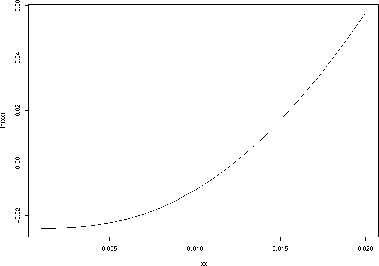
One of the things uniroot does not do well is find roots where the sign does not change on either side:
> uniroot(function(xx)xx^2,c(-0.1,0.1)) Error in uniroot(function(xx) xx^2, c(-0.1, 0.1)) : f() values at end points not of opposite sign |
Sometimes it can handle deranged functions:
> fn <- function(x1) {
+   xx<-x1-0.01
+   ww <- 100*(abs(xx*sin(1/xx)))^2+ xx*xx
+   ww[is.na(ww)] <- 0
+   ww[xx<0] <- (-1)*ww[xx<0]
+   ww
+ }
> xs <- seq(-0.1,0.1,by=0.0001)
> plot(xs,fn(xs),type="l")
> abline(h=0)
> uniroot(fn,c(-0.1,0.1))
$root
[1] 0.009997432

$f.root
[1] -4.6764e-10

$iter
[1] 16

$estim.prec
[1] 6.103516e-05
|
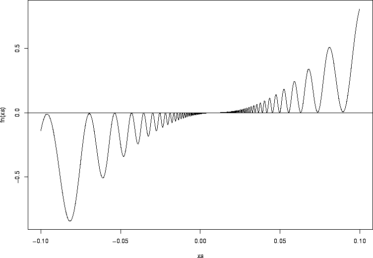 Numerical analysis texts are full of strange functions that can wreak havoc
on your root finder.
So we used the root finder uniroot to find how small the true infection probability could be and still be in a sense consistent with 3 infections out of 51. We decided that we would reject the hypothesis that the infection probability was (say) 0.001, since if it were that small, there would be too small a chance of seeing as many as three infections. We solved to find out for what infection probability would the chance of seeing three or more infections reach 2.5%.
Now, let's go the other way. How big could it be and still be consistent with as few as three infections? We know that as the infection probability per injury gets bigger and bigger, the chance of getting only 3 or fewer infections should get quite small. Let's plot it:
> xx <- seq(0,0.2,by=0.001) > ww <- pbinom(3,prob=xx,size=51) > plot(xx,ww,type="l") > abline(h=0.025) |
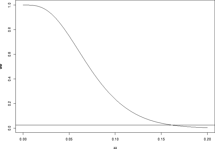
> uniroot(function(xx)pbinom(3,prob=xx,size=51)-0.025, + c(0.001,0.999)) $root [1] 0.1624314 $f.root [1] -9.51687e-06 $iter [1] 10 $estim.prec [1] 6.103516e-05 |
So what we have done is to compute the best estimate, 0.0588, together with an exact 95% confidence interval, (0.0123, 0.162). Confidence intervals determined by this method are called Clopper-Pearson exact confidence intervals1.
We can construct a function to compute these intervals, as follows:
> cp.lower <- function(xx,nn,alpha=0.025,low=1e-6,hi=1-1e-6) {
+   uniroot(function(pp){1-pbinom(xx-1,size=nn,prob=pp)-alpha},c(low,hi))$root
+ }
> cp.upper <- function(xx,nn,alpha=0.025,low=1e-6,hi=1-1e-6) {
+   uniroot(function(pp){pbinom(xx,size=nn,prob=pp)-alpha},c(low,hi))$root
+ }
> cp.interval <- function(xx,nn,alpha=0.05,low=1e-6,hi=1-1e-6) {
+   c(cp.lower(xx,nn,alpha/2,low=low,hi=hi),
+     cp.upper(xx,nn,alpha/2,low=low,hi=hi))
+ }
> cp.interval(xx=3,nn=51)
[1] 0.01230367 0.16243854
|
With the functions we just defined, we can actually compute one-sided upper confidence bounds too. What do you do when you find no successes? Suppose that out of 9 injuries, we found no infections. Based on just these data, our best estimate of the probability is the observed fraction 0/9, but we certainly can't just stop there. The fact that there are only nine subjects should mean that this estimate is not all that precise. So let's compute a 95% upper confidence limit, using the function above:
> # continuing... > cp.upper(0,9,alpha=0.05) [1] 0.2831307 |
The binomial confidence interval can actually be expressed in terms of an exact formula2:
> cp.interval.lt <- function(xx,nn,alpha=0.05,low=1e-6,hi=1-1e-6) {
+ # I'm keeping the arguments low and hi in place so this function will
+ #   be interchangeable with the other
+   f1<-qf(alpha/2,df1=2*xx,df2=2*(nn-xx+1))
+   f2<-qf(1-alpha/2,df1=2*(xx+1),df2=2*(nn-xx))
+   b1 <- 1+(nn-xx+1)/(xx*f1)
+   b2 <- 1+(nn-xx)/((xx+1)*f2)
+   c(1/b1,1/b2)
+ }
> cp.interval.lt(xx=3,nn=51)
[1] 0.01229909 0.16242222
|
For another example, consider the results of a study of hepatotoxicity and INH (isoniazid) preventive therapy for latent tuberculosis infection3. In Table 3, the investigators reported the rate of hepatotoxicity as a number of cases per 1000 persons starting therapy. Let's compute exact confidence intervals where appropriate, and where the rate is zero, let's compute a one-sided upper confidence limit. First, I'm going to shine up the confidence interval function in a few ways: I'm going to make it able to generate confidence intervals if you give a vector of alphas. And I'm going to make it be able to handle a vector of different possible numerators and denominators (but if you give it a vector of alphas and a vector of numerators or denominators, I'm going to make it complain). I'm also going to arrange for it to automatically report a 95% one-sided upper limit if the count is zero. Exercise: modify this to report 95% one-sided lower limit if the numerator equals the denominator. Finally, I'm going to report the result as a matrix rather than a list, to make it easier to scale the results by 1000 the way the authors did, and I'm also going to include the best estimate (the observed counts over the number of trials).
> age.numerators <- c(0,6,4,1)
> age.denominators <- c(1468,7449,1865,359)
> age.rates <- age.numerators/age.denominators
> cp.interval.lt <- function(xx,nn,alpha=0.05,low=1e-6,hi=1-1e-6) {
+    alen <- length(alpha)
+    xlen <- length(xx)
+    nlen <- length(nn)
+    if (alen>1 && (xlen>1 || nlen>1)) {
+      stop("error--cp.interval.lt has wrong input lengths.")
+    }
+    if (alen>1) {
+      if (xx>0) {
+        f1<-qf(alpha/2,df1=2*xx,df2=2*(nn-xx+1))
+        f2<-qf(1-alpha/2,df1=2*(xx+1),df2=2*(nn-xx))
+        b1 <- 1+(nn-xx+1)/(xx*f1)
+        b2 <- 1+(nn-xx)/((xx+1)*f2)
+        lowers <- 1/b1
+        uppers <- 1/b2
+      } else {
+        f2<-qf(1-alpha,df1=2*(xx+1),df2=2*(nn-xx))
+        b2 <- 1+(nn-xx)/((xx+1)*f2)
+        lowers <- rep(0,alen)
+        uppers <- 1/b2
+      }
+    } else {
+      inputs <- rbind(xx=xx,nn=nn)
+      nc <- ncol(inputs)
+      xx <- inputs["xx",]
+      nn <- inputs["nn",]
+      lowers <- rep(NA,nc)
+      uppers <- rep(NA,nc)
+      for (ii in 1:nc) {
+        if (xx[ii]>0) {
+          f1<-qf(alpha/2,df1=2*xx[ii],df2=2*(nn[ii]-xx[ii]+1))
+          f2<-qf(1-alpha/2,df1=2*(xx[ii]+1),df2=2*(nn[ii]-xx[ii]))
+          b1 <- 1+(nn[ii]-xx[ii]+1)/(xx[ii]*f1)
+          b2 <- 1+(nn[ii]-xx[ii])/((xx[ii]+1)*f2)
+          lowers[ii] <- 1/b1
+          uppers[ii] <- 1/b2
+        } else {
+          lowers[ii] <- 0
+          f2<-qf(1-alpha,df1=2*(xx[ii]+1),df2=2*(nn[ii]-xx[ii]))
+          b2 <- 1+(nn[ii]-xx[ii])/((xx[ii]+1)*f2)
+          uppers[ii] <- 1/b2
+        }
+      }
+    }
+    rbind(uppers=uppers,lowers=lowers,estimate=xx/nn)
+  }
> cps <- 1000*cp.interval.lt(age.numerators,age.denominators)
> cps
             [,1]      [,2]      [,3]        [,4]
uppers   2.038609 1.7523542 5.4822852 15.42143959
lowers   0.000000 0.2956515 0.5846777  0.07052066
estimate 0.000000 0.8054772 2.1447721  2.78551532
> gen.ci.plot <- function(cps,xaxis,xticks) {
+   mx <- max(cps)
+   ngrp <- ncol(cps)
+   plot(1:ngrp,cps["estimate",],col="red",ylim=c(0,mx),
+            xlab=xaxis,
+            ylab="Rate per 1000 Persons starting therapy",type="n",axes=FALSE)
+   axis(1,at=1:ngrp,labels=xticks)
+   axis(2)
+   box()
+   points(1:ngrp,cps["uppers",],col="blue")
+   points(1:ngrp,cps["lowers",],col="blue")
+   points(1:ngrp,cps["estimate",],col="red")
+   for (ii in 1:ngrp) {
+     lines(x=c(ii,ii),y=cps[c("lowers","uppers"),ii],col="black")
+   }
+   cps
+ }
> age.cps <- gen.ci.plot(cps,"Patient Age",c("0-14","15-34","35-64","65+"))
> age.cps <- gen.ci.plot(cps,"Patient Age",c("0-14","15-34","35-64","65+"))
> eth.cps <- gen.ci.plot(1000*cp.interval.lt(c(4,7,5,2,0,0),c(1856,9285,5968,1732,1050,535)),"Ethnicity",c("\"White\"","\"Nonwhite\"","\"Asian\"","\"Black\"","\"Hispanic\"","\"Other\""))
> sex.cps <- gen.ci.plot(1000*cp.interval.lt(c(3,8),c(6066,5075)),"Sex",c("Male","Female"))
> age.cps
             [,1]      [,2]      [,3]        [,4]
uppers   2.038609 1.7523542 5.4822852 15.42143959
lowers   0.000000 0.2956515 0.5846777  0.07052066
estimate 0.000000 0.8054772 2.1447721  2.78551532
> eth.cps
              [,1]      [,2]      [,3]      [,4]     [,5]     [,6]
uppers   5.5088248 1.5527099 1.9540574 4.1650110 2.849012 5.583852
lowers   0.5875144 0.3031606 0.2720861 0.1398743 0.000000 0.000000
estimate 2.1551724 0.7539041 0.8378016 1.1547344 0.000000 0.000000
> sex.cps
              [,1]     [,2]
uppers   1.4446268 3.103672
lowers   0.1020017 0.680796
estimate 0.4945598 1.576355
|
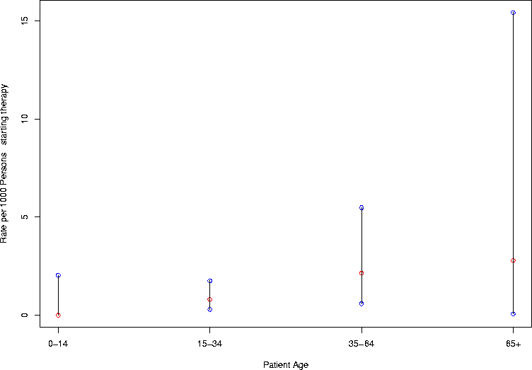
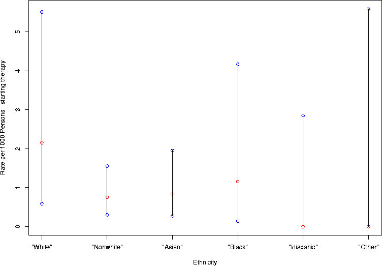
Exercise. Use the manual page (?text) regarding the function text to figure out how to print the number of subjects at the top of each confidence bar.
It might also be useful to see the probability of getting 0 cases out of the 1468 individuals aged 0-14. Here is how to plot such a graph. In this case, I color the line red, so it will stand out from the dotted lines I used to draw the lines indicating where 5%, 10%, and 20% were (what true hepatotoxicity rates corresponded to a 5%, 10%, and 20% chance of seeing no cases in the patients). How do these values relate to the one-sided confidence limits for different type-I error rates?
npatients <- 1468
> xscale <- 1000
> xs <- seq(0,0.005,by=0.00005)
> ps <- dbinom(0,size=npatients,prob=xs)
> plot(xscale*xs,ps,type="l",xlab=paste("True Rate of Hepatotoxicity as Cases per",xscale,"starting therapy"),ylab=paste("Probability of zero cases in",npatients,"patients"),col="red")
> for (pct in c(0.05,0.1,0.2)) {
+   loc <- uniroot(function(xx)(dbinom(0,size=npatients,prob=xx)-pct),c(0,0.1),tol=1e-6)
+   cury <- dbinom(0,size=npatients,prob=loc$root)
+   lines(x=xscale*rep(loc$root,2),y=c(-0.1,cury),lty=2)
+   lines(x=xscale*c(-0.14,loc$root),y=rep(cury,2),lty=2)
+   curx <- xscale*loc$root
+   text(curx,cury+0.05,as.character(round(curx,digits=2)))
+ }
|
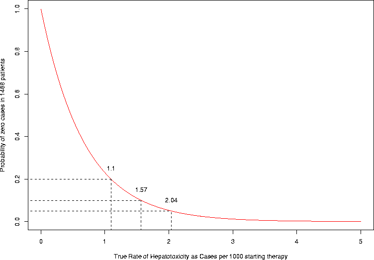
Exercise. Find the 99% upper confidence limit using the same procedure as above. Ans. 3.13.
We could simulate the needlestick incident 100 times, assuming that the probability of needlestick is in reality 3/51:
> rbinom(100,size=51,prob=3/51) [1] 5 4 2 0 2 7 0 2 1 3 4 2 4 4 6 3 6 4 3 3 3 3 2 0 4 1 5 6 1 3 1 5 3 1 3 1 8 [38] 3 2 4 3 4 3 6 2 4 2 4 3 3 5 4 4 2 4 4 2 4 2 1 1 1 4 4 4 3 4 1 1 5 2 0 4 1 [75] 3 7 2 5 2 3 0 2 2 6 0 5 4 4 2 2 3 2 3 1 2 2 3 0 4 4 |
That's all for today. Next time we'll continue with examples.
1 Clopper CJ, Pearson ES. The use of confidence or fiducial limits illustrated in the case of the binomial. Biometrika 26:404-413, 1934.
2 Leemis LM, Trivedi KS. A comparison of approximate interval estimators for the Bernoulli parameter. American Statistician 50:63-68, 1996.
3 Nolan CM, Goldberg SV, Buskin SE. Hepatotoxicity associated with Isoniazid preventive therapy. A 7-year survey from a public health tuberculosis clinic. Journal of the American Medical Association 281(11):1014-1018, 1999.