Quantiles

A q-quantile is defined to be the smallest x such that the chance of a random variable being greater than or equal to x is at least q.

The meaning of this is easier to see in the concrete. Let's look back at the binomial again. Let's first plot the cumulative distribution function for the needle example, where the number of trials was 51 and the success probability 0.03:

> plot(plot(0:10,pbinom(0:10,size=51,prob=0.03),ylim=c(0,1)) > abline(h=0.25) > pbinom(0:10,size=51,prob=0.03) [1] 0.2115234 0.5451634 0.8031325 0.9334468 0.9818109 0.9958714 0.9992053 [8] 0.9998681 0.9999809 0.9999976 0.9999997

Notice that we set the vertical range to (0,1) manually by using ylim, and then placed a horizontal line in the figure using abline. Now, the chance of getting a zero is 0.211 or so, and the chance of getting a one is about 0.334, of getting a two is about 0.260, and a three is about 0.130. Cumulatively, the chance of being less than or equal to zero (pbinom) is 0.211, less than or equal to one about 0.545, less than or eaual to two about 0.803, and so on. What is the 0.25-quantile of this distribution? We want to know what X value corresponds to 25% of the distribution being below it; how big does x have to be to be sure that you have at least a 25% chance of being below x? How about 0? Not good enough, since you only have a 21.1% (or so) chance of being at or below 0 (at 0, here, since you can't be less than 0). What about 1? In this case, P(X>=1) is 0.545, which is at least 0.25. For all other possible values of x, this probability is also greater than 0.25, but 1 is the smallest such value. This is as small an x you can get and just go over; you have to have an x of 1 to be sure that at least 25% of the probability is at or below 1.

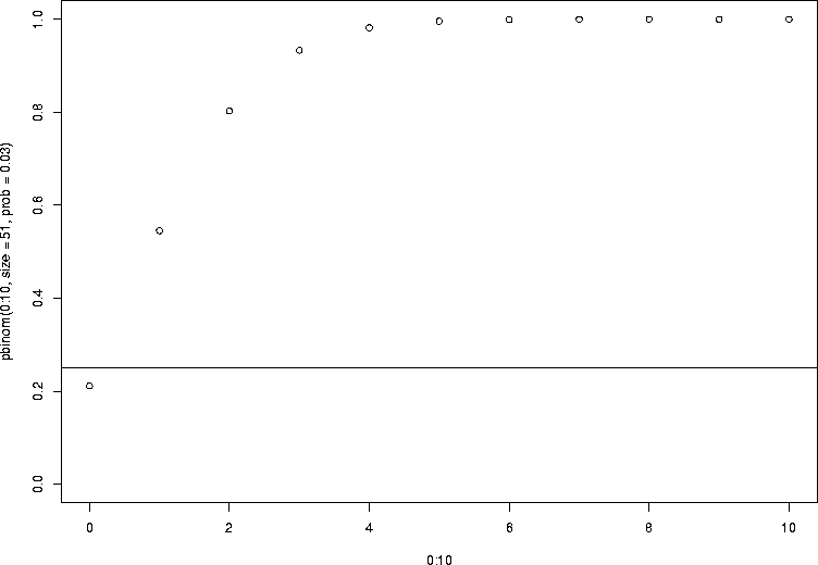
> qbinom(0.25,size=51,prob=0.03) [1] 1

So the purpose of the quantile function is to tell you where to draw the cutoffs to make sure you have a certain amount of the distribution on the left hand side. This is quite easy for a continuous random variable like the standard normal:

> qnorm(0.025) [1] -1.959964 > qnorm(c(0.005,0.01,0.025,0.05,0.1,0.5,0.9,0.95,0.975,0.99,0.995)) [1] -2.575829 -2.326348 -1.959964 -1.644854 -1.281552 0.000000 1.281552 [8] 1.644854 1.959964 2.326348 2.575829

So the chance of a standard normal being less than or equal to (same answer as the chance of being less than) about -1.96 is 0.025; -1.96 is where to put the cutoff so as to have a 2.5% chance of being on the left.

R has built in quantile functions for all sorts of useful distributions that come up in statistics, eliminating the need for tables:

> qchisq(0.95,df=1) [1] 3.841459 > qt(0.025,df=10) [1] -2.228139 > qf(0.95,df1=3,df2=37) [1] 2.858796

So you see the chi-square distribution, t-distribution, and F-distributions. R has many other distributions as well, such as Poisson, beta, gamma, and negative binomial.

Confidence limits

Last time we spent some time talking about "exact" confidence intervals for the Binomial distribution. We observe a certain number X of successes in N independent idential bernoulli trials, and compute the observed frequency of success, X/N. And this value X/N estimates the true success probability. We found how to compute an interval estimate of this using the binomial distribution. Every time we do the experiment, we should get a different number of successes in principle, since this is a random variable, and therefore we should get a different confidence interval. The confidence interval is a random variable, and the idea is that it should have a certain chance of containing the true value. Let's simulate this process, as follows:

> cp.interval.lt <- function(xx,nn,alpha=0.05,low=1e-6,hi=1-1e-6) { + f1<-qf(alpha/2,df1=2*xx,df2=2*(nn-xx+1)) + f2<-qf(1-alpha/2,df1=2*(xx+1),df2=2*(nn-xx)) + b1 <- 1+(nn-xx+1)/(xx*f1) + b2 <- 1+(nn-xx)/((xx+1)*f2) + c(1/b1,1/b2) + } > contains.val <- function(cis,a.value) { + (a.value > cis$lower) & (a.value < cis$upper) + } > gen.intervals <- function(xxs,size,nvals=length(xxs)) { + lowers <- rep(NA,nvals) + uppers <- rep(NA,nvals) + for (ii in 1:nvals) { + intvl <- cp.interval.lt(xxs[ii],size,alpha=0.05) + lowers[ii] <- intvl[1] + uppers[ii] <- intvl[2] + } + lowers[is.nan(lowers)] <- -1 + list(lowers=lowers,uppers=uppers) + } > nn <- 20000 > nsims<-10000 > tru <- 0.5 > sum(contains.val(gen.intervals(rbinom(nsims,size=nn,prob=tru),nn), tru)) [1] 9535

So first we do this with a binomial with twenty thousand trials (N is 20000), and a true probability of success of 50%. (Think of tossing two hundred dollars worth of pennies.) We count up the number of heads (successes) and compute the relative frequency, and then use the formula for the exact confidence limit. We determine whether or not the confidence interval contains the true value 0.5, and then we do this ten thousand times. How many times did the confidence interval contain 0.5? As you see, it contained it a little over 95% of the time (95.35% to be exact)...not too bad. We retry it now with N equal to 51 and p equal to 0.03:

> # continuing example from above > sum(contains.val( + gen.intervals(rbinom(nsims,size=nn,prob=tru),nn), tru + )) [1] 9805 There were 50 or more warnings (use warnings() to see the first 50) Rweb:> warnings() Warning messages: 1: NaNs produced in: qf(p, df1, df2, lower.tail, log.p)

Question: why did we generate NaN's, and why did we worry about the value of lowers in this case? What do you think about setting lowers to -1?